An Approach to Mathematic Functions Basics

by Frank C. Fung ( 1st published in December, 2014. )

Top Of Page

Section XII - Equation of the Hyperbola in [ Polar Co-ordinates ]

Summary for the Section :

• In this Section , we shall derive the equation for the Hyperbola in [ Polar co-ordinates ] ,
  • i.e. , this equation :
    • 

go to Top Of Page

Polar Co-ordinates explained :

• In general , if the point [ Point P ] is a point on the Hyperbola , then :
  • its position is defined by the position-vector [ Vector O-P ] ,

    where :

    • [ Point O ] is the point-of-origin at the intersection of the [ U-Axis ] and the [ V-Axis ] .

  And the position-vector [ Vector O-P ] is defined by two (2) variables :

  • the distance [ RHO ] :
    • 

  • the angle [ THETA ] :
    • 

go to Top Of Page

Preparing for the Derivation Process :

• Again , we take note that :
  • for the Hyperbola we have developed in Section VIII ,
    • the relevent range of [ u ] is :
      • 

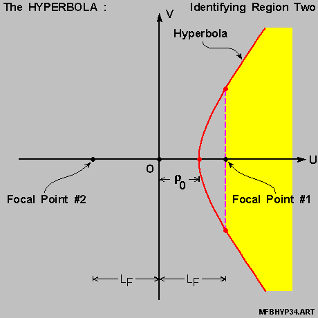
  We shall again split this { relevent range of [ u ] } into two (2) sub-regions :

  • [ Region One ] being the region where :
    • 

  • [ Region Two ] being the region where :
    • 

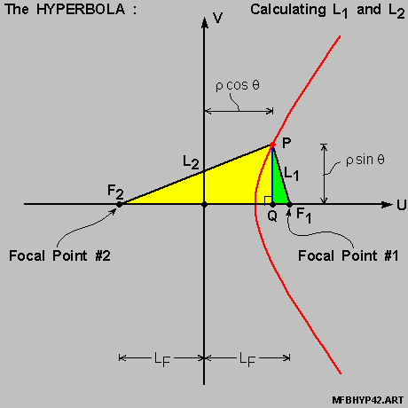
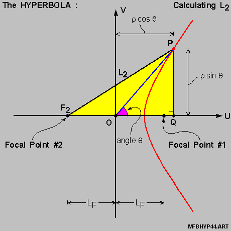
    as per this set of 2 diagrams below .

  

  The reasoning here for the splitting is the same as before in Section IX ;

  • namely that the set-up for [ L1 ] and [ L2 ] will be slightly different for the 2 regions .

go to Top Of Page

Calculating [ L1 ] and [ L2 ] in [ Region One ] :

• Let us now take a quick look at the set-up for [ L1 ] and [ L2 ] in [ Region One ] ,
  • and we identify the point [ Point P ] as any point on the Hyperbola within this sub-region ,
    • as per the diagram on-the-left below .

  

  We then have , for the diagram on-the-right above :

  • for [ Right-Angle Triangle F1-Q-P ] :
    • 

  • for [ Right-Angle Triangle F2-Q-P ] :
    • 

go to Top Of Page

Calculating [ L1 ] and [ L2 ] in [ Region Two ] :

• Let us now take a quick look at the set-up for [ L1 ] and [ L2 ] in [ Region Two ] ,
  • and we identify the point [ Point P ] as any point on the Hyperbola within this sub-region .

  

  We then have :

  • for [ Right-Angle Triangle F1-Q-P ] in the diagram on-the-left above :
    • 

  • for [ Right-Angle Triangle F2-Q-P ] in the diagram on-the-right above :
    • 

go to Top Of Page

Consolidating [ Region One ] and [ Region Two ] :

• We see here that the equations for [ L2 ] are the same for both regions here ,
  • i.e. , this equation :
    • 

      is in fact common to both .

  But the equations for [ L1 ] are slightly different ;

  • for [ Region One ] :
    • 

  • for [ Region Two ] :
    • 

  However , these 2 equations immediately above are different in format only ,

  • and are in-essence the same equation .

• Thus , we can use either of these equations in our development process to follow ,
  • and we shall now elect to use the first equation here from-here-on-in .

  As such we can now write :

  • 

    yielding :

  • 

  And this shall be the core equation we shall be using for our development process , next .

go to Top Of Page

Developing the equation for the Hyperbola :

• We now bring back the core equation from immediately above :
  • 

  Re-arranging terms then yields :

  • 

• Let us now take a closer look at the algebraic terms under the [ square-root sign ] :
  • For the terms under the [ square-root sign ] on the left-hand-side , we have :
    • 

      yielding :

    • 

  • For the terms under the [ square-root sign ] on the right-hand-side , we have :
    • 

      yielding :

    • 

  Let us now plug-in these results back into the orginal equation , and we have :

  • 

• Let us square both sides of the equation to arrive at this :
  • 

    

  And on rearranging and cancelling terms , we have :

  • 

  Further re-arrangements then yield us this equation :

  • 

  Let us now divided throughout by [ 2*D ] , and we have :

  • 

    yielding :

  • 

• Let us now square both sides of the equation to arrive at this :
  • 

  And on cancelling terms , we have :

  • 

• Let us recall , at this point , that we have already established this relation :
  • 

    towards the end of Section VIII .

  Therefore :

  • 

  Substituting this into the equation immediately preceding then yields us this :

  • 

    yielding :

  • 

• Further re-arrangements then yield us this equation :
  • 

  And consequently ,

  • 

  Further munipulations then yield us the same equation in this format :

  • 

    yielding :

  • 

  We shall now divide throughout by { [ L-sub-F ]-square } , and we have :

  • 

    yielding :

  • 

• Let us now introduce the quantity [ ALPHA ] such that :
  • 

  or ,

  • 

  We can then re-write the equation immediately preceding in this format :

  • 

  Consequently :

  • 

    yielding further this relation :

  • 

• And the final equation derived therefrom is then :
  • 

go to Top Of Page

go to the next section : Section XIII - The Hyperbola via [ Focal-Point Based Co-ordinates ] - Part I

go to the last section : Section XI - Equation of the Hyperbola in [ U-V Axis Co-ordinates ]

return to the MATH Functions Basics HomePage

Original dated 2014-12-07